Custom Search
|
|
  |
|
|
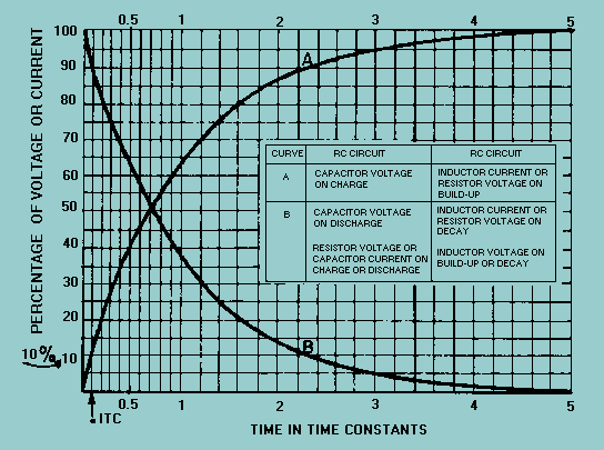
INTEGRATOR WAVEFORM ANALYSIS If either an RC or RL circuit has a time constant 10 times greater than the duration of the input pulse, the circuits are capable of integration. Let's compute and graph the actual waveform that would result from a long time constant (10 times the pulse duration), a short time constant (1/10 of the pulse duration), and a medium time constant (that time constant between the long and the short). To accurately plot values for the capacitor output voltage, we will use the Universal Time Constant Chart shown in figure 4-34. Figure 4-34. - Universal Time Constant Chart.
You already know that capacitor charge follows the shape of the curve shown in figure 4-34. This curve may be used to determine the amount of voltage across either component in the series RC circuit. As long as the time constant or a fractional part of the time constant is known, the voltage across either component may be determined.
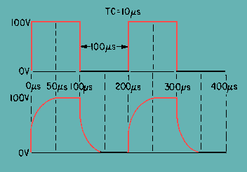
Short Time-Constant Integrator In figure 4-35, a 100-microsecond pulse at an amplitude of 100 volts is applied to the circuit. The circuit is composed of the, 0.01mF capacitor and the variable resistor, R. The square wave applied is a pure square wave. The resistance of the variable resistor is set at a value of 1,000 ohms. The time constant of the circuit is given by the equation: TC = RC Substituting values: T = 1,000 0.01mF T = (1 X 10³) (1 X-8) T = 1 X 10⁻⁵ vor 10 microseconds Figure 4-35. - RC integrator circuit.
Since the time constant of the circuit is 10 microseconds and the pulse duration is 100 microseconds, the time constant is short (1/10 of the pulse duration). The capacitor is charged exponentially through the resistor. In 5 time constants, the capacitor will be, for all practical purposes, completely charged. At the first time constant, the capacitor is charged to 63.2 volts, at the second 86.5 volts, at the third 95 volts, at the fourth 98 volts, and finally at the end of the fifth time constant (50 microseconds), the capacitor is fully charged. This is shown in figure 4-36. Figure 4-36. - Square wave applied to a short time-constant integrator.
Notice that the leading edge of the square wave taken across the capacitor is rounded. If the time constant were made extremely short, the rounded edge would become square. Medium Time-Constant Integrator The time constant, in figure 4-36 can be changed by increasing the value of the variable resistor (figure 4-35) to 10,000 ohms. The time constant will then be equal to 100 microseconds. This time constant is known as a medium time constant. Its value lies between the extreme ranges of the short and long time constants. In this case, its value happens to be exactly equal to the duration of the input pulse, 100 microseconds. The output waveform, after several time constants, is shown in figure 4-37. The long, sloping rise and fall of voltage is caused by the inability of the capacitor to charge and discharge rapidly through the 10,000-ohm series resistance. Figure 4-37. - Medium time-constant integrator.
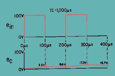
At the first instant of time, 100 volts is applied to the medium time-constant circuit. In this circuit, 1TC is exactly equal to the duration of the input pulse. After 1TC the capacitor has charged to 63.2 percent of the input voltage (100 volts). Therefore, at the end of 1TC (100 microseconds), the voltage across the capacitor is equal to 63.2 volts. However, as soon as 100 microseconds has elapsed, and the initial charge on the capacitor has risen to 63.2 volts, the input voltage suddenly drops to 0. It remains there for 100 microseconds. The capacitor will now discharge for 100 microseconds. Since the discharge time is 100 microseconds (1TC), the capacitor will discharge 63.2 percent of its total 63.2-volt charge, a value of 23.3 volts. During the next 100 microseconds, the input voltage will increase from 0 to 100 volts instantaneously. The capacitor will again charge for 100 microseconds (1TC). The voltage available for this charge is the difference between the voltage applied and the charge on the capacitor (100 - 23.3 volts), or 76.7 volts. Since the capacitor will only be able to charge for 1TC, it will charge to 63.2 percent of the 76.7 volts, or 48.4 volts. The total charge on the capacitor at the end of 300 microseconds will be 23.3 + 48.4 volts, or 71.7 volts. Notice that the capacitor voltage at the end of 300 microseconds is greater than the capacitor voltage at the end of 100 microseconds. The voltage at the end of 100 microseconds is 63.2 volts, and the capacitor voltage at the end of 300 microseconds is 71.7 volts, an increase of 8.5 volts. The output waveform in this graph (eC) is the waveform that will be produced after many cycles of input signal to the integrator. The capacitor will charge and discharge in a step-by-step manner until it finally charges and discharges above and below a 50-volt level. The 50-volt level is controlled by the maximum amplitude of the symmetrical input pulse, the average value of which is 50 volts. Long Time-Constant Integrator If the resistance in the circuit of figure 4-35 is increased to 100,000 ohms, the time constant of the circuit will be 1,000 microseconds. This time constant is 10 times the pulse duration of the input pulse. It is, therefore, a long time-constant circuit. The shape of the output waveform across the capacitor is shown in figure 4-38. The shape of the output waveform is characterized by a long, sloping rise and fall of capacitor voltage. Figure 4-38. - Square wave applied to a long time-constant integrator.
At the first instant of time, 100 volts is applied to the long time-constant circuit. The value of charge on the capacitor at the end of the first 100 microseconds of the input signal can be found by using the Universal Time Constant Chart (figure 4-34). Assume that a line is projected up from the point on the base line corresponding to 0.1TC. The line will intersect the curve at a point that is the percentage of voltage across the capacitor at the end of the first 100 microseconds. Since the applied voltage is 100 volts, the charge on the capacitor at the end of the first 100 microseconds will be approximately 9.5 volts. At the end of the first 100 microseconds, the input signal will fall suddenly to 0 and the capacitor will begin to discharge. It will be able to discharge for 100 microseconds. Therefore, the capacitor will discharge 9.5 percent of its accumulated 9.5 volts (.095 X 9.5 = 0.90 volt). The discharge of the 0.90 volt will result in a remaining charge on the capacitor of 8.6 volts. At the end of 200 microseconds, the input signal will again suddenly rise to a value of 100 volts. The capacitor will be able to charge to 9.5 percent of the difference (100 - 8.6 = 91.4 volts). This may also be figured as a value of 8.7 volts plus the initial 8.6 volts. This results in a total charge on the capacitor (at the end of the first 300 microseconds) of 8.7 + 8.6 = 17.3 volts. Notice that the capacitor voltage at the end of the first 300 microseconds is greater than the capacitor voltage at the end of the first 100 microseconds. The voltage at the end of the first 100 microseconds is 9.5 volts; the capacitor voltage at the end of the first 300 microseconds is 17.3 volts, an increase of 7.8 volts. The capacitor charges and discharges in this step-by-step manner until, finally, the capacitor charges and discharges above and below a 50-volt level. The 50-volt level is controlled by the maximum amplitude of the square-wave input pulse, the average value of which is 50 volts. Q.21 What is the numerical difference (in terms of the time constant) between a long
and a short time-constant circuit? |
|
|
|
Integrated Publishing, Inc. - A (SDVOSB) Service Disabled Veteran Owned Small Business
|