GRAPHICAL ANALYSIS OF THE BASIC CIRCUIT

One of the most valuable methods of analyzing a circuit is by constructing a graph. No other method provides a more convenient or more rapid way to observe the characteristics of an electrical device.

The first step in constructing a graph is to obtain a table of data. The information in the table can be obtained by taking measurements on the circuit under examination, or can be obtained theoretically through a series of Ohm's law computations. The latter method is used here.

Since there are three variables (E, I, and R) to be analyzed, there are three distinct graphs that may be constructed.

To construct any graph of electrical quantities, it is standard practice to vary one quantity in a specified way and note the changes which occur in a second quantity. The quantity which is intentionally varied is called the independent variable and is plotted on the horizontal axis. The horizontal axis is known as the X-AXIS. The second quantity, which varies as a result of changes in the first quantity, is called the dependent variable and is plotted on the vertical, or Y-AXIS. Any other quantities involved are held constant.

For example, in the circuit shown in figure 3-6, if the resistance was held at 10 ohms and the voltage was varied, the resulting changes in current could then be graphed. The resistance is the constant, the voltage is the independent variable, and the current is the dependent variable.

Figure 3-6. - Three variables in a basic circuit.

Figure 3-7 shows the graph and a table of values. This table shows R held constant at 10 ohms as E is varied from 0 to 20 volts in 5-volt steps. Through the use of Ohm's law, you can calculate the value of current for each value of voltage shown in the table. When the table is complete, the information it contains can be used to construct the graph shown in figure 3-7. For example, when the voltage applied to the 10-ohm resistor is 10 volts, the current is 1 ampere. These values of current and voltage determine a point on the graph. When all five points have been plotted, a smooth curve is drawn through the points.

Figure 3-7. - Volt-ampere characteristic.

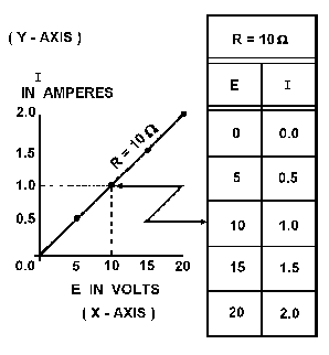
Through the use of this curve, the value of current through the resistor can be quickly determined for any value of voltage between 0 and 20 volts.

Since the curve is a straight line, it shows that equal changes of voltage across the resistor produce equal changes in current through the resistor. This fact illustrates an important characteristic of the basic law - the current varies directly with the applied voltage when the resistance is held constant.

When the voltage across a load is held constant, the current depends solely upon the resistance of the load. For example, figure 3-8 shows a graph with the voltage held constant at 12 volts. The independent variable is the resistance which is varied from 2 ohms to 12 ohms. The current is the dependent variable. Values for current can be calculated as:

Figure 3-8. - Relationship between current and resistance.



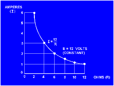
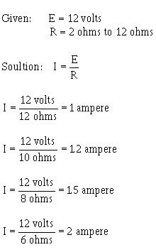
This process can be continued for any value of resistance. You can see that as the resistance is halved, the current is doubled; when the resistance is doubled, the current is halved.

This illustrates another important characteristic of Ohm's law - current varies inversely with resistance when the applied voltage is held constant.

Using the graph in figure 3-7,
what is the approximate value of current when the voltage is 12.5 volts?

Using the graph in figure 3-8,
what is the approximate value of current when the resistance is 3 ohms?