With integral control, the final control element's position changes at a rate determined by the amplitude of the input error signal. Recall that:

Error = Setpoint - Measured Variable

If a large difference exists between the setpoint and the measured variable, a large error results. This causes the final control element to change position rapidly. If, however, only a small difference exists, the small error signal causes the final control element to change position slowly.

Figure 20 illustrates a process using an integral controller to maintain a constant flow rate. Also included is the equivalent block diagram of the controller.

instrumentation%20and%20control_files/image315.jpg">

Figure 20 Integral Flow Rate Controller

Initially, the system is set up on an anticipated flow demand of 50 gpm, which corresponds to a control valve opening of 50%. With the setpoint equal to 50 gpm and the actual flow measured at 50 gpm, a zero error signal is sent to the input of the integral controller. The controller output is initially set for a 50%, or 9 psi, output to position the 6-in control valve to a position of 3 in open. The output rate of change of this integral controller is given by:

instrumentation%20and%20control_files/image317.jpg">

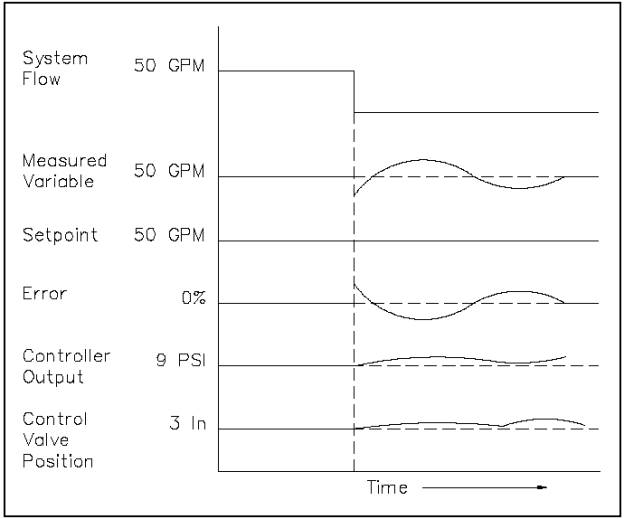
If the measured variable decreases from its initial value of 50 gpm to a new value of 45 gpm, as seen in Figure 21, a positive error of 5% is produced and applied to the input of the integral controller. The controller has a constant of 0.1 seconds^-', so the controller output rate of change is 0.5% per second.

The positive 0.5% per second indicates that the controller output increases from its initial point of 50% at 0.5% per second. This causes the control valve to open further at a rate of 0.5% per second, increasing flow.

Figure 21 Reset Controller Response

The controller acts to return the process to the setpoints. This is accomplished by the repositioning of the control valve. As the controller causes the control valve to reposition, the measured variable moves closer to the setpoint, and a new error signal is produced. The cycle repeats itself until no error exists.

The integral controller responds to both the amplitude and the time duration of the error signal. Some error signals that are large or exist for a long period of time can cause the final control element to reach its "fully open" or "fully shut" position before the error is reduced to zero. If this occurs, the final control element remains at the extreme position, and the error must be reduced by other means in the actual operation of the process system.

Properties of Integral Control

The major advantage of integral controllers is that they have the unique ability to return the controlled variable back to the exact setpoint following a disturbance.

Disadvantages of the integral control mode are that it responds relatively slowly to an error signal and that it can initially allow a large deviation at the instant the error is produced. This can lead to system instability and cyclic operation. For this reason, the integral control mode is not normally used alone, but is combined with another control mode.

Summary

integral controllers are summarized below.

Integral Control Summary

An integral controller provides an output rate of change that is determined by the magnitude of the error and the integral constant.

The controller has the unique ability to return the process back to the exact setpoint.

The integral control mode is not normally used by itself because of its slow response to an error signal.